Many of the blocks in GNU Radio allow the user to select what data type (complex, float, int, byte, etc.) the block operates on. Writing a new block to handle each data type would be tedious, so the framework includes a utility to generate a number of different blocks from template files. I’ve used this to handle different data types in my message utility blocks and some research projects. While useful, I haven’t seen a lot of out-of-tree projects use it so I thought I’d add a step-by-step guide to using the utility for your own out-of-tree blocks.

Background

One may notice that many of the blocks in GNU Radio Companion include an option to configure the data type (complex, float, int, byte, etc.) that the block uses, often with a parameter called “IO Type”:

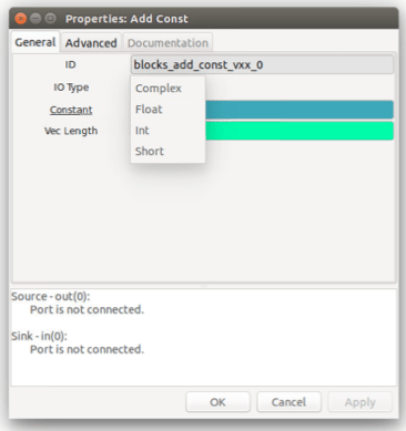
The Add Const block supports several data types

Looking at the relevant parts in the block’s XML definition file we see that the option is used to call a different block for each data type

blocks.add_const_v$(type.fcn)($const)
...
 <param>
   <name>IO Type</name>
   <key>type</key>
   <type>enum</type>
   <option>
     <name>Complex</name>
     <key>complex</key>
     <opt>const_type:complex_vector</opt>
     <opt>fcn:cc</opt>
   </option>
   <option>
     <name>Float</name>
     <key>float</key>
     <opt>const_type:real_vector</opt>
     <opt>fcn:ff</opt>
   </option>
...

For example, selecting the complex option causes GNU Radio to call blocks.add_const_vcc whereas the float option will call blocks.add_const_vff. So where are those defined?

Though they are separate blocks in the view of GNU Radio, each was generated from a common file. Looking in the gnuradio/gr-blocks/lib directory we see the files add_const_vXX_impl.cc.t and add_const_vXX_impl.h.t which are the template files for each block. There is a similar add_const_vXX.h.t in the gnuradio/gr-blocks/include/gnuradio/blocks directory. Taking a look at the CMakeLists.txt shows the commands to generate the blocks.

include(GrMiscUtils)
GR_EXPAND_X_H(blocks add_const_vXX bb ss ii ff cc)

At compile time, the appropriate files will be generated from the templates and compiled. After that, they can be called from a Python or GNU Radio companion like any other block.

Let’s Build Our Own

There are a few steps to using the utility in your own out-of-tree projects, so let’s go through them step-by-step. Following the steps of the GNU Radio tutorial for writing out-of-tree modules we’ll create a block that performs a simple squaring operation. We’ll go through the process step-by-step, but the end result can be downloaded from GitHub to save some typing.

The new module was created using gr_modtool newmod howtogen. After that, the template files square_XX.h.t, square_XX_impl.cc.t, and square_XX_impl.h.t were added. Let’s take a look at those, beginning with square_XX.h.t:

#ifndef @GUARD_NAME@
#define @GUARD_NAME@
#include <howtogen/api.h>
#include <gnuradio/sync_block.h>

namespace gr {
  namespace howtogen {

    class HOWTOGEN_API @NAME@ : virtual public gr::sync_block
    {
     public:
      typedef boost::shared_ptr<@NAME@> sptr;
      static sptr make();
    };

  } // namespace howtogen
} // namespace gr

#endif /* @GUARD_NAME@ */

When generating files, the utility will replace @NAME@ with the appropriate class name: square_ff for the float case, square_cc for the complex, and so on. Looking in the work function of square_XX_impl.cc.t we see similar variables:

int
@NAME_IMPL@::work(int noutput_items,
          gr_vector_const_void_star &input_items,
          gr_vector_void_star &output_items)
{
    @I_TYPE@ *in = (@I_TYPE@ *) input_items[0];
    @O_TYPE@ *out = (@O_TYPE@ *) output_items[0];
    for(int ii=0;ii<noutput_items;ii++)
    {
      out[ii] = in[ii]*in[ii];
    }
    return noutput_items;
}

The utility will replace @I_TYPE@ and @O_TYPE@ with the correct data types: byte, int, float, etc. @NAME_IMPL@ will be the same as @NAME@ but with _impl at the end, as in square_ff_impl. To summarize, here is a list of the macros when translated for the float case:

An XML file is created that allows the user to call the appropriate block from a user-selectable parameter in GNU Radio. A part of that is shown below:

<make>howtogen.square_$(type.fcn)()</make>
<param>
    <name>IO Type</name>
    <key>type</key>
    <type>enum</type>
    <option>
        <name>Complex</name>
        <key>complex</key>
        <opt>fcn:cc</opt>
    </option>
    ...

That gets all our files in place. What’s left to do is instruct the compiler how to expand and install the generated blocks. We’ll edit include/howtogen/CMakeLists.txt:

include(GrMiscUtils)
GR_EXPAND_X_H(howtogen square_XX             ss ii ff cc bb)

add_custom_target(howtogen_generated_includes DEPENDS
    ${generated_includes}
)

install(FILES
    api.h
    ${generated_includes}
    DESTINATION include/howtogen
)

GrMiscUtils is included in the make file and the GR_EXPAND_X_H macro tells the module name, the header file template name, and then lists what data types to expand with. These files will be generated as ${generated_includes} so we’ll need to tell CMake to install those. Similar instructions are added to lib/CMakeLists.txt:

include(GrPlatform) #define LIB_SUFFIX

include(GrMiscUtils)
GR_EXPAND_X_CC_H_IMPL(howtogen square_XX ss ii ff cc bb)

include_directories(${Boost_INCLUDE_DIR})
link_directories(${Boost_LIBRARY_DIRS})

list(APPEND howtogen_sources
    ${generated_sources}
)

set(howtogen_sources "${howtogen_sources}" PARENT_SCOPE)
if(NOT howtogen_sources)
    MESSAGE(STATUS "No C++ sources... skipping lib/")
    return()
endif(NOT howtogen_sources)

add_library(gnuradio-howtogen SHARED ${howtogen_sources})
add_dependencies(gnuradio-howtogen howtogen_generated_includes howtogen_generated_swigs)
target_link_libraries(gnuradio-howtogen ${Boost_LIBRARIES} ${GNURADIO_ALL_LIBRARIES})
set_target_properties(gnuradio-howtogen PROPERTIES DEFINE_SYMBOL "gnuradio_howtogen_EXPORTS")

We’ll again include GrMiscUtils and use the GR_EXPAND_X_CC_H_IMPL macro to generate the appropriate files. We’ll need to add {$generated_sources}to the sources and finally add howtogen_generated_inlcudes and howtogen_generated_swigs as dependencies using add_depedencies.

The next step is to add the files to howtogen_swig.i. There’s no macro to expand these, so we’ll type in each filename manually.

#define HOWTOGEN_API
%include "gnuradio.i"            // the common stuff
%include "howtogen_swig_doc.i"
%{
#include "howtogen/square_bb.h"
#include "howtogen/square_ss.h"
#include "howtogen/square_ii.h"
#include "howtogen/square_ff.h"
#include "howtogen/square_cc.h"
%}

%include "howtogen/square_bb.h"
%include "howtogen/square_ss.h"
%include "howtogen/square_ii.h"
%include "howtogen/square_ff.h"
%include "howtogen/square_cc.h"

GR_SWIG_BLOCK_MAGIC2(howtogen, square_bb);
GR_SWIG_BLOCK_MAGIC2(howtogen, square_ss);
GR_SWIG_BLOCK_MAGIC2(howtogen, square_ii);
GR_SWIG_BLOCK_MAGIC2(howtogen, square_ff);
GR_SWIG_BLOCK_MAGIC2(howtogen, square_cc);

Lastly, we’ll edit the howtogen_swig.i file to include the following lines:

file(GLOB xml_files "*.xml")

install(FILES
    ${xml_files} DESTINATION share/gnuradio/grc/blocks
)

Now everything should be in place to build. The Git repo contains some unit tests to ensure the square operation performs correctly. There is also a GNU Radio Companion flow graph to test if the XML generation worked correctly.

In a previous post I talked about the process of using both MATLAB and GNU Radio to process data in real time. I recently used this process to put together a demonstration on how you could use an RTL-SDR to sense and decode the information your Keyless Entry remote sends to your car. This is a pretty popular demonstration of software-defined radio, Adam Laurie and Balint Seeber have put together similar demos.

Eventually I want to get the entire thing working with just GNU Radio but the hybrid approach is working well for now. It also shows how such a hybrid approach might be useful for other software-defined radio applications.

The Background

Keyless remote entry systems have been around for a while and likely aren’t going away any time soon. Your remote can send commands to your car wirelessly using a small radio transmitter to tell your car to unlock, lock, etc.

These remotes vary between auto manufacturers but for the most part they transmit at 315MHz and use On-Off Keying (OOK), a very simple form of digital modulation. OOK sends an RF signal of a certain length to represent a ‘1’ and stays silent to represent a ‘0’.

For security reasons the remote doesn’t send the same signal each time. The remote encrypts its commands using a rolling key so the bits representing each command are different each time. Your car and remote share the same private key which makes it so only your car can decode the encrypted transmission.

This begs the question, what happens when I press a button when I’m out of range of my car? Doesn’t that get the two rolling keys out of sync? Your car actually calculates the rolling key for the next transmission it expects as well as the next 256 transmissions (that number may vary between manufacturers). If any of the 256 match the received signal from your remote, the car will unlock and resynchronize. Of course, if you use your remote more than 256 times while out of range of your car the two will get out of sync. In that case there is usually a procedure in the owner’s manual to get them synced up again.

The Setup

To receive the signal I’ll use an RTL-SDR dongle tuned to 315MHz and running at the default sample rate of 2Msps. In GNU Radio I’ll decimate and lowpass filter the received signal. Since the modulation is OOK, I will just take the magnitude of the received signals.

That data will be written into a FIFO as previously discussed. I will continue the rest of the processing in MATLAB.

Getting The Bits 

In MATLAB I will begin by opening and reading samples from the FIFO. As per the previous post, I’ll make sure that I start the flow graph running before trying to read samples from the FIFO, or MATLAB will lock up.

fi = fopen('data/keyless_mag_fifo','rb');
raw = fread(fi, buffer_len, 'float');

This will give a chunk of floating point samples of length buffer_len (in this case 50,000) containing transmissions and silence. I’ll use a simple energy detection to figure out the start of the frame.

50,000 samples captured from the RTL-SDR, showing two transmissions.

eng_mat = vec2mat(raw,10);
x_mag = abs(eng_mat).^2;
x_sum = sum(x_mag,2);

b = x_sum(2:end);
a = x_sum(1:end-1);

x_diff = b./a;
x_norm = x_diff./max(x_diff);

The stream is broken up into chunks of ten samples. The energy of each chunk is calculated by taking the sum of the magnitude squared. Two vectors containing the calculated energies are created with the vector a lagging one chunk behind the vector b. If I divide b by a the resulting vector x_diff will contain peaks when the transmissions begin.

Result of energy detection run on the 50,000 samples.

x_ind = find(x_norm>threshold);
if (isempty(x_ind))
    x_ind = 1;
end

start_ind = x_ind(1)*window_len;

If I then normalize the vector x_diff so that the tallest peak has a value of 1, I can set a threshold (0.2 in this case) that I’ll consider the start of the peak. If I find a peak I can calculate the sample with which to start the packet.

Normalized energy detection with threshold. I’ll detect the two packets, but process one at a time 

I’ll then count out a number of samples after the start index (in this case 6,000) and save that as the packet. I’ll do a quick check that I have at least 6,000 samples left in the vector raw. If not, I’ll check if there are more samples available in the buffer and grab those. I’ll then remove those samples from the vector raw.

The first packet in raw, containing 6,000 samples

if (start_ind+pkt_len)>length(raw)
    in_buff = fread(fi, buffer_len, 'float');
    if (isempty(in_buff))
        %display('Buffer Empty')
        continue
    end
    raw = cat(1,raw,in_buff);
end

x_pkt = raw(start_ind:start_ind+pkt_len);
raw = raw(start_ind+pkt_len+1:end);

After processing these samples I’ll return to read 6,000 more samples from raw until the vector is empty at which point I’ll grab 50,000 more samples from the buffer and store it in raw.

At this point I can take a closer look at the packet extracted from raw. Looking at the first 250 samples I can see the on-off keying more clearly.

Raw packet, zoomed in on the first 250 samples

I’ll then filter the signal with an integrator to smooth out the plateaus and silences that comprise the OOK signal.

x_filt = filter(ones(1,n)/n,1,x_pkt);

Filtered packet, zoomed in on the first 250 samples

Then I’ll use a threshold to filter the further so each sample is either a one or a zero.

x_dec = x_filt;
x_dec(x_dec>0.3) = 1;
x_dec(x_dec~=1) = 0;

In this case the threshold used is 0.3. I’ll then cut the beginning of the packet so that the first sample is the start of the first plateau.

x_ind = find(x_dec);
if (isempty(x_ind))
    continue;
end

start_ind = x_ind(1);
x_dec = x_dec(start_ind:end);

Data after threshold, zoomed in on the first 250 samples

Next I need to convert the OOK pulses into bits. For this I’ll count the duration of the plateaus and silences.

counter =0;
bit_ind = 1;
for ii=2:length(x_dec)-1
    if (x_dec(ii)~=x_dec(ii-1)) % Transition
        counter = 0;
    else
        counter=counter+1;
        if (counter>16)
            counter=0;
            bit(bit_ind) = x_dec(ii);
            bit_ind=bit_ind+1;
        end
    end
end

After a high-low or low-high transition we’ll start a counter. If the counter reaches a value (16 in this case) without another transition occurring I’ll store the bit.

The first 250 samples yield the first 12 bits of the data

The bits can then be converted to bytes using MATLAB’s bi2de function.

bit_group = vec2mat(bit,8);
byte = bi2de(bit_group)';

Decoding The Signal

The last part is to make sense of all the bytes that are being transmitted. In addition to the encryption mentioned above, the format of the packet is almost entirely different for each car manufacturer. The structure below pertains to my Saturn, but your car may be different.

I found the packet starts off with thirteen bytes of value 85 (alternating ones and zeros in binary) to synchronize the transmission. I start by finding these bytes and keeping everything after them as the payload.

known_sync = 85*ones(1,13);
if (length(byte)<14)
    continue
end
sync = byte(1:13);
payload = byte(14:end);

If the sync is found I flag the packet as good and go on to display the results. If the sync wasn’t correctly found I skip this packet and go back to the start of the loop to grab more data.

pkt_good = false;
if (isequal(sync,known_sync))
    display('Received Pkt')
    pkt_good=true;
end
if (~pkt_good)
    continue
end

Unfortunately due to the encryption this is where the decoding stops. What I have next is a sequence of approximately 20 bytes that correspond to a command transmitted to my car. However, due to the encryption I cannot tell what command is being sent. Instead I just display the sync code and the data along with a message that the signal was received. The data stays around for a few seconds and then fades.

Next Steps

While this project shows a good example of using both MATLAB and GNU Radio, for this particular application it would probably be best to use one or the other. I would like to eventually transition all the signal processing over to GNU Radio. My other option would be to interface directly with the RTL-SDR in MATLAB using the Communication Systems Toolbox to control the RTL-SDR. Processing the data using MATLAB’s object-oriented programming features would also improve the efficiency, but that might just have to be a project for another day.

Until then, the code for this project can be found on GitHub.